Practical Applications

1 Introduction

Broadcasting comes up frequent enough in real world problems. This page gives a few examples of these.

2 Binding arrays along an arbitrary dimension

The abind() function, from the package of the same name, allows one to bind arrays along any arbitrary dimensions (not just along rows or columns).
Unfortunately, abind() does not support broadcasting, which can lead to frustrations such as the following:

x <- array(1:27, c(3,3,3))
y <- array(1L, c(3,3,1))
abind::abind(x, y, along = 2)

#> Error in abind(x, y, along = 2) : 
#>  arg 'X2' has dims=3, 3, 1; but need dims=3, X, 3

Here, abind() is complaining about the dimensions not fitting perfectly.
But intuitively, binding x and y should be possible, with dimension 3 from array y being broadcasted to size 3.

The bind_array() function provided by the ‘broadcast’ package can bind the arrays without problems:

x <- array(1:27, c(3,3,3))
y <- array(1L, c(3,3,1))
bind_array(list(x, y), 2)
#> , , 1
#> 
#>      [,1] [,2] [,3] [,4] [,5] [,6]
#> [1,]    1    4    7    1    1    1
#> [2,]    2    5    8    1    1    1
#> [3,]    3    6    9    1    1    1
#> 
#> , , 2
#> 
#>      [,1] [,2] [,3] [,4] [,5] [,6]
#> [1,]   10   13   16    1    1    1
#> [2,]   11   14   17    1    1    1
#> [3,]   12   15   18    1    1    1
#> 
#> , , 3
#> 
#>      [,1] [,2] [,3] [,4] [,5] [,6]
#> [1,]   19   22   25    1    1    1
#> [2,]   20   23   26    1    1    1
#> [3,]   21   24   27    1    1    1

bind_array() is also considerably faster and more memory efficient than abind().

3 Vector quantization

Here is an example taken from Numpy’s own online documentation.

The basic operation in Vector Quantization (VQ) finds the closest point in a set of points, called codes in VQ jargon, to a given point, called the observation. In the very simple, two-dimensional case shown below, the values in observation describe the weight and height of an athlete to be classified. The codes represent different classes of athletes. Finding the closest point requires calculating the distance between observation and each of the codes. The shortest distance provides the best match. In this example, codes[1] is the closest class indicating that the athlete is likely a basketball player.


observation <- array(c(111.0, 188.0), dim = c(1, 2))
codes <- array(
  c(102.0, 203.0,
    132.0, 193.0,
    45.0, 155.0,
    57.0, 173.0),
  dim = c(4, 2)
)

diff <- bc.d(codes, observation, "-") # broadcasting happens here
dist <- matrixStats::colSums2(diff^2) |> sqrt()
which.min(dist) |> print()
#> [1] 1
codes[1] |> print()
#> [1] 102

4 Perform computation on all possible pairs

Suppose you have 2 vectors of character strings, and you want to concatenate all possible pairs of these strings.

In base , this would require a either a loop (which is slow), or repeating the vectors several times (which requires more memory).

The ’broadcasted way to do this, is to make the vectors orthogonal, and concatenate the strings of the orthogonal vectors - this is both fast and memory efficient.

For example:

x <- array(letters[1:10], c(10, 1))
y <- array(letters[1:10], c(1, 10))

out <- bc.str(x, y, "+")
dimnames(out) <- list(x, y)
print(out)
#>   a    b    c    d    e    f    g    h    i    j   
#> a "aa" "ab" "ac" "ad" "ae" "af" "ag" "ah" "ai" "aj"
#> b "ba" "bb" "bc" "bd" "be" "bf" "bg" "bh" "bi" "bj"
#> c "ca" "cb" "cc" "cd" "ce" "cf" "cg" "ch" "ci" "cj"
#> d "da" "db" "dc" "dd" "de" "df" "dg" "dh" "di" "dj"
#> e "ea" "eb" "ec" "ed" "ee" "ef" "eg" "eh" "ei" "ej"
#> f "fa" "fb" "fc" "fd" "fe" "ff" "fg" "fh" "fi" "fj"
#> g "ga" "gb" "gc" "gd" "ge" "gf" "gg" "gh" "gi" "gj"
#> h "ha" "hb" "hc" "hd" "he" "hf" "hg" "hh" "hi" "hj"
#> i "ia" "ib" "ic" "id" "ie" "if" "ig" "ih" "ii" "ij"
#> j "ja" "jb" "jc" "jd" "je" "jf" "jg" "jh" "ji" "jj"

5 Grouped Broadcasting

5.1 Casting with equal group sizes

Suppose you read the following matrix from a file:

x <- cbind(
  id = rep(1:3, each = 2),
  grp = rep(1:2, 3),
  val = 1:6 * 2
)
print(x)
#>      id grp val
#> [1,]  1   1   2
#> [2,]  1   2   4
#> [3,]  2   1   6
#> [4,]  2   2   8
#> [5,]  3   1  10
#> [6,]  3   2  12

For computing purposes, you may need the rows of each group - defined in column “grp” - to be cast to a new dimension. This is commonly needed to perform a grouped broadcasted operation.

‘broadcast’ allows users to cast subsets of an array onto a new dimension, based on some grouping factor. In this case, the following will do the job:

margin <- 1L # we cast from the rows, so margin = 1
grp <- as.factor(x[, 2]) # factor to define which rows belongs to which group
levels(grp) <- c("a", "b") # names for the new dimension
out <- acast(x, margin, grp) # casting is performed here
broadcaster(out) <- TRUE
print(out)
#> , , a
#> 
#>      id grp val
#> [1,]  1   1   2
#> [2,]  2   1   6
#> [3,]  3   1  10
#> 
#> , , b
#> 
#>      id grp val
#> [1,]  1   2   4
#> [2,]  2   2   8
#> [3,]  3   2  12
#> 
#> broadcaster

Notice that the dimension-names of the new dimension (dimension 3) are equal to levels(grp).

With the cast array, one can use broadcasting to easily do things like multiply the values in each group with a different value, like so:


# create the multiplication factor array:
mult <- array(
  1, c(1, 3, 2),
  list(NULL, c("mult_id", "mult_grp", "mult_val"), c("a", "b"))
)
mult[, "mult_val", c("a", "b")] <- c(2, 10)
broadcaster(mult) <- TRUE
print(mult)
#> , , a
#> 
#>      mult_id mult_grp mult_val
#> [1,]       1        1        2
#> 
#> , , b
#> 
#>      mult_id mult_grp mult_val
#> [1,]       1        1       10
#> 
#> broadcaster

# grouped broadcasted operation:
out2 <- out * mult
dimnames(out2) <- dimnames(out)
print(out2)
#> , , a
#> 
#>      id grp val
#> [1,]  1   1   4
#> [2,]  2   1  12
#> [3,]  3   1  20
#> 
#> , , b
#> 
#>      id grp val
#> [1,]  1   2  40
#> [2,]  2   2  80
#> [3,]  3   2 120
#> 
#> broadcaster

Perhaps you’d like to reverse-cast the array back when you’re done computing; reverse-casting an array can be done be combining asplit() with bind_array():

asplit(out2, ndim(out2)) |> bind_array(along = margin)
#>     id grp val
#> a.1  1   1   4
#> a.2  2   1  12
#> a.3  3   1  20
#> b.1  1   2  40
#> b.2  2   2  80
#> b.3  3   2 120

…though the order of, in this case, the rows (because margin = 1) will not necessarily be the same as the original array.

5.2 Casting with unequal group sizes

The casting arrays also works when the groups have unequal sizes, though there are a few things to keep in mind.

Let’s start again with the input array:

x <- cbind(
  id = c(rep(1:3, each = 2), 1),
  grp = c(rep(1:2, 3), 2),
  val = rnorm(7)
)
print(x)
#>      id grp        val
#> [1,]  1   1 -1.9974838
#> [2,]  1   2 -0.4981739
#> [3,]  2   1 -0.7033263
#> [4,]  2   2  0.2066804
#> [5,]  3   1 -1.0600505
#> [6,]  3   2 -0.7654767
#> [7,]  1   2 -0.3455591

Once again, the acast() to fill the gaps, otherwise an error is called.

Thus one can cast in this case like so:

grp <- as.factor(x[, 2])
levels(grp) <- c("a", "b")
margin <- 1L
out <- acast(x, margin, grp, fill = TRUE)
print(out)
#> , , a
#> 
#>      id grp        val
#> [1,]  1   1 -1.9974838
#> [2,]  2   1 -0.7033263
#> [3,]  3   1 -1.0600505
#> [4,] NA  NA         NA
#> 
#> , , b
#> 
#>      id grp        val
#> [1,]  1   2 -0.4981739
#> [2,]  2   2  0.2066804
#> [3,]  3   2 -0.7654767
#> [4,]  1   2 -0.3455591

Notice that some values are missing ( NA ); if some groups have unequal number of elements, acast() needs to fill the gaps with missing values. By default, gaps are filled with NA if x is atomic, and with list(NULL) if x is recursive. The user can change the filling value through the fill_value argument.

Once again, we can get the original array back when we’re done like so:

asplit(out, ndim(out)) |> bind_array(along = margin)
#>     id grp        val
#> a.1  1   1 -1.9974838
#> a.2  2   1 -0.7033263
#> a.3  3   1 -1.0600505
#> a.4 NA  NA         NA
#> b.1  1   2 -0.4981739
#> b.2  2   2  0.2066804
#> b.3  3   2 -0.7654767
#> b.4  1   2 -0.3455591

… but we do keep the missing values when the groups have an unequal number of elements.

6 Manually compute confidence/credible interval for a spline

The sd_lc() function computes the standard deviation for a linear combination of random variables. One of its notable use-cases is to compute the confidence interval (or credible interval if you’re going Bayesian) of a spline.

Packages like ‘mgcv’ provides the user to plot and analyse the smoothers with confidence from a fitted GAM.
But not all packages are as user-friendly. So one practical application of sd_lc() is computing confidence intervals of splines when a package does not provide that service in a user-friendly way.

Please note that the sd_lc() functions is just a linear algebra function, not specific to any type/class of model; so this function assumes you know what you’re doing.

For a demonstration of sd_lc(), the following will be done:

a GAM model will be fitted using the ‘mgcv’ package. The model will consist of several low-rank thin-plate (lrtp) smoothers.
One of these lrtp splines will be plotted with credible intervals using the plot() method provided by ‘mgcv’ itself.
The sd_lc() function will be used to re-create compute the credible intervals of the spline from step 2 and re-create the plot.

For the sake of this demonstration, I’ll forgo some crucially mandatory steps in statistical modelling - like data exploration, model diagnostics, and model interpretation.

First, let’s create some data, fit a GAM on it, and plot the spline for variable “x2”:

d <- mgcv::gamSim(7, n = 1000L, dist = "normal", scale = 2L)
#> Gu & Wahba 4 term additive model, correlated predictors
m <- mgcv::gam(y ~ s(x1) + s(x2) + s(x3), data = d)
par(mfrow = c(1,1))
plot(m, select = 2)

Now extract the required model parameters to recreate this plot:


# get names of relevant coefficients:
coeffnames <- names(coef(m))
coeffnames <- coeffnames[grepl("x2", coeffnames)]
print(coeffnames)
#> [1] "s(x2).1" "s(x2).2" "s(x2).3" "s(x2).4" "s(x2).5" "s(x2).6" "s(x2).7"
#> [8] "s(x2).8" "s(x2).9"

# get necessary model parameters (i.e. X, b, vc)
# but only for relevant coefficients:
b <- coef(m)[coeffnames]
X <- predict(m, type="lpmatrix")[, coeffnames, drop = FALSE]
vc <- vcov(m)[coeffnames, coeffnames, drop = FALSE]

Computing the means of the spline is trivial:

means <- X %*% b

Computing the (~ 95%) credible interval is a bit trickier - at least if you want to avoid unnecessary copies/memory-usage when you have a large dataset, and don’t want to use a slow for-loop.
But using the sd_lc() function it becomes relatively easy to compute it very memory-efficiently, even with a very large dataset:


st.devs <- sd_lc(X, vc) # get standard deviations efficiently
mult <- 2 # mgcv uses multiplier of 2; approx. 95% credible interval
lower <- means - mult * st.devs
upper <- means + mult * st.devs

Now let’s plot the manually computed spline over the original one, and see how well our own estimate fits.
I’ll use transparent green dots for the mean, and transparent red dots for the credible interval:

# defines some colours:
colour1 <- rgb(red = 0, green = 1, blue = 0, alpha = 0.15)
colour2 <- rgb(red = 1, green = 0, blue = 0, alpha = 0.15)

# original plot from the 'mgcv' R-package:
par(mfrow = c(1,1))
plot(m, select = 2)

# our own re-creation plotted over it:
lc <- data.frame(
  x = d$x2,
  means = means,
  lower = lower,
  upper = upper
)
lc <- lc[order(lc$x),]
points(x = lc$x, y = lc$mean, col = colour1) # plot our means
points(x = lc$x, y = lc$lower, col = colour2) # plot our lower bound
points(x = lc$x, y = lc$upper, col = colour2) # plot our upper bound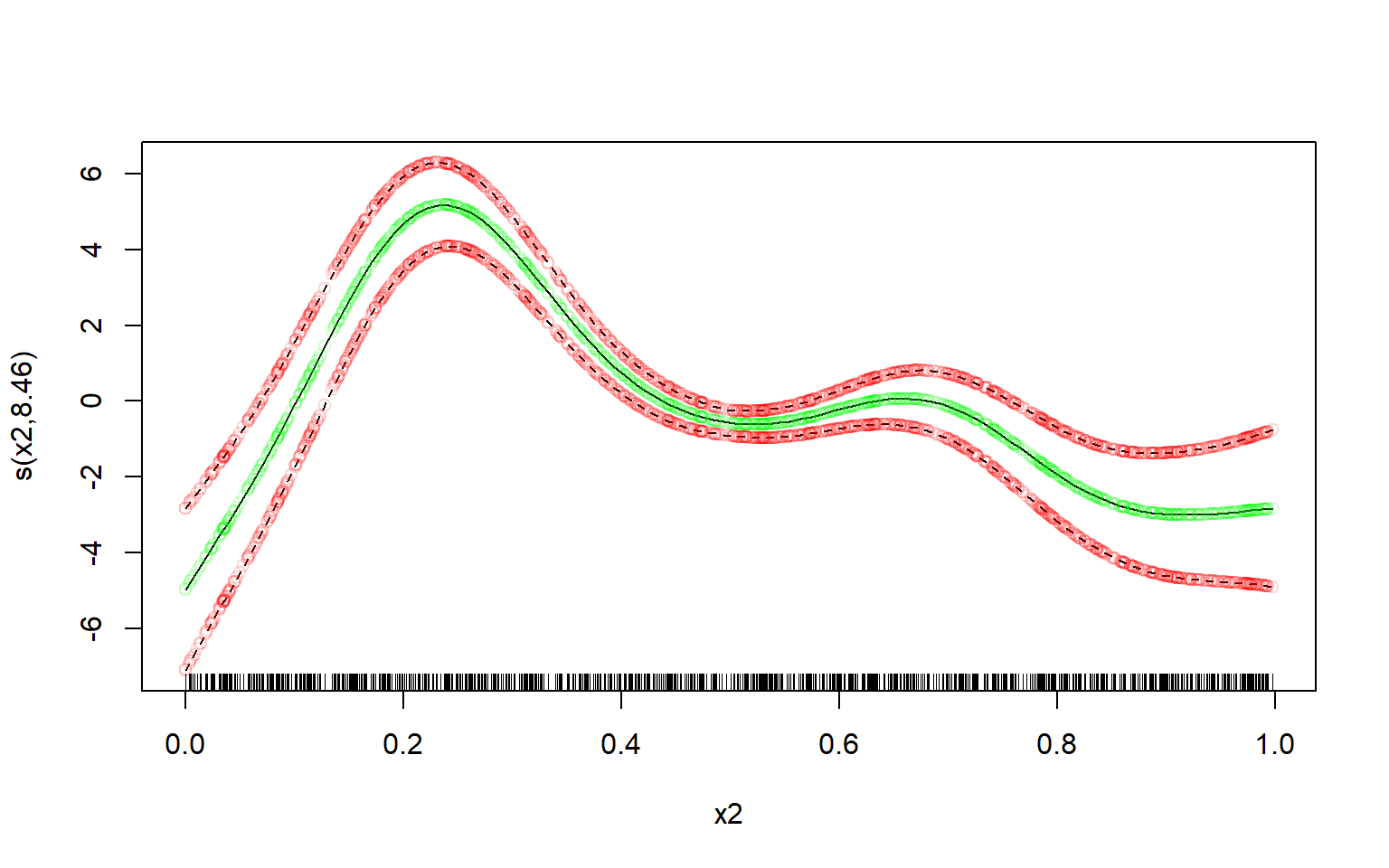

Perfect fit.

Since one can very easily re-create the plot using sd_lc(), one can also use a different plotting framework altogether.
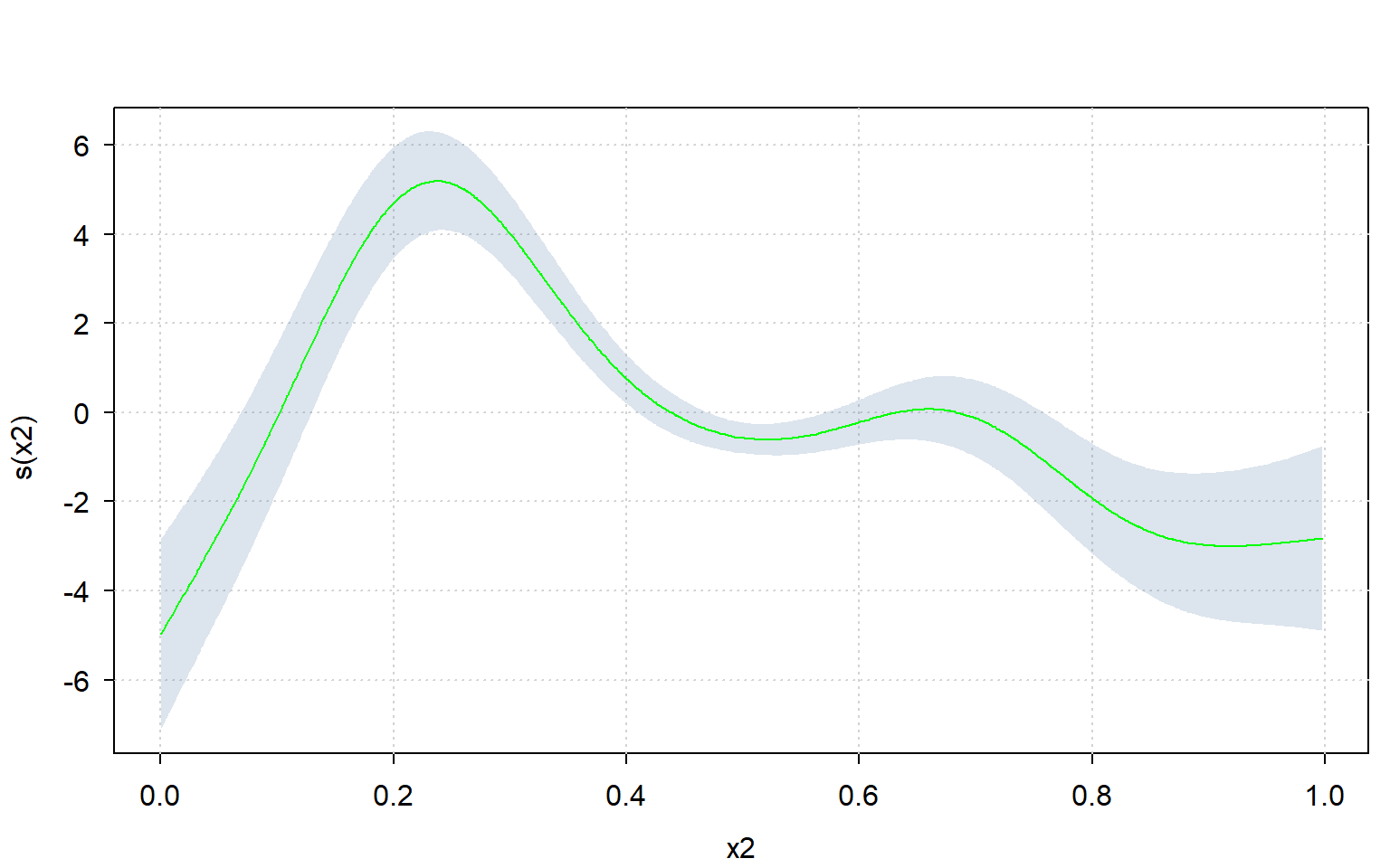
Let’s use the ‘tinyplot’ framework to compute the plot manually:

library(tinyplot)
#> Warning: package 'tinyplot' was built under R version 4.4.2
tinytheme("clean")
tinyplot( # plot confidence interval
  x = lc$x, ymin = lc$lower, ymax = lc$upper, type = "ribbon",
  xlab = "x2", ylab = "s(x2)",
)
tinyplot( # plot means over it
  x = lc$x, y = lc$means, type = "l",
  add = TRUE, col = "green"
)