# import sys
# !{sys.executable} -m pip install numpy --upgrade
# set-up #
import numpy as np
import gc
from time import perf_counter
def myfunc(a, b):
a + b
# end set-up #
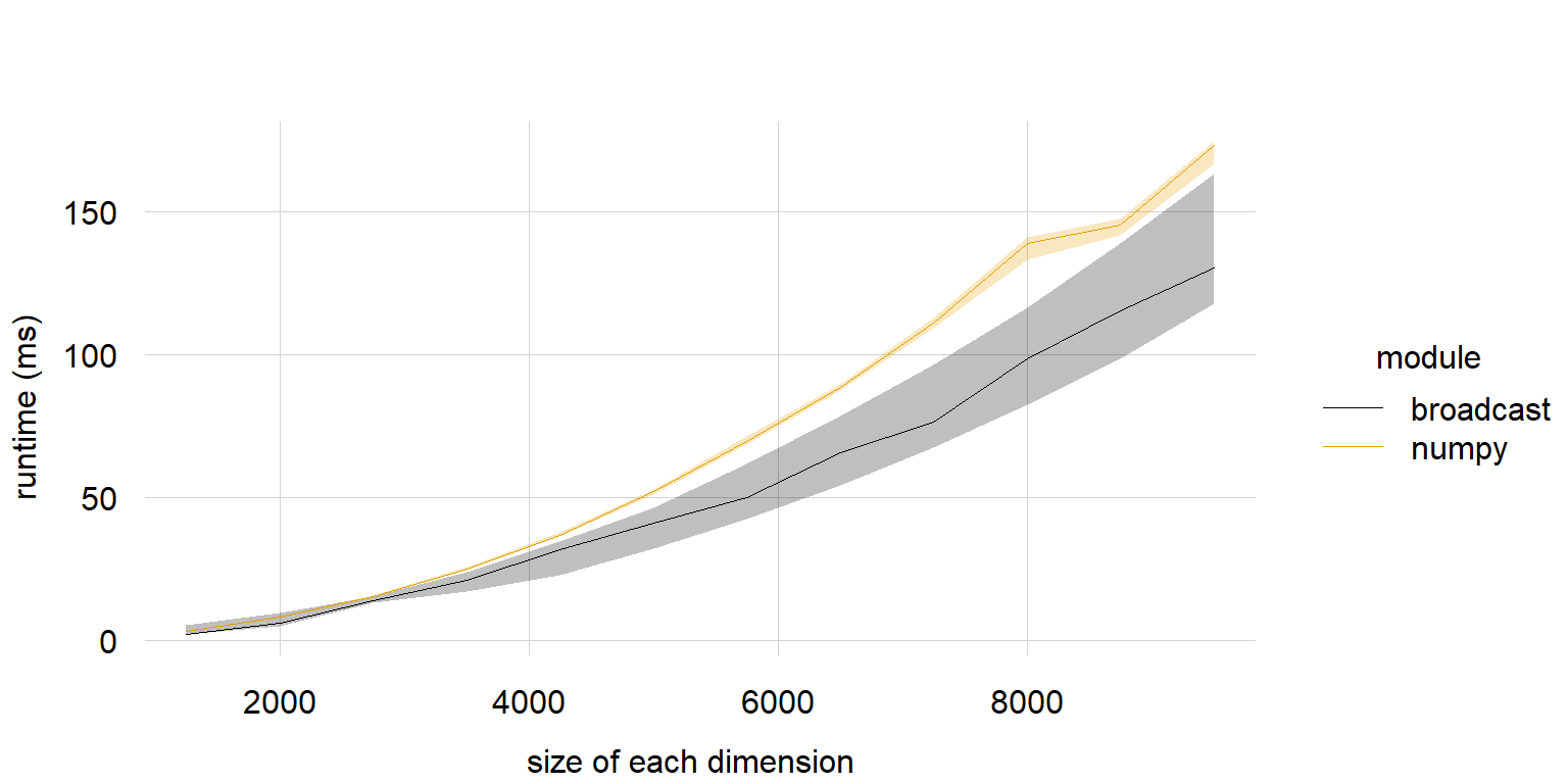
# 2d array #
print("2d")
gc.disable()
dimsizes = np.arange(1250, 9501, 750)
median_np = np.zeros(len(dimsizes))
q1_np = np.zeros(len(dimsizes))
q3_np = np.zeros(len(dimsizes))
durations = np.zeros(100)
for i in range(0, len(dimsizes)):
print(i)
n = dimsizes[i]
adims = (n, 1)
bdims = (1, n)
x = np.random.random_sample(adims)
y = np.random.random_sample(bdims)
for j in range(0, len(durations)):
t1_start = perf_counter()
myfunc(x, y)
t1_stop = perf_counter()
durations[j] = (t1_stop-t1_start) * 1000
durations2 = durations[10:]
median_np[i] = np.median(durations2)
q1_np[i] = np.quantile(durations2, 0.25)
q3_np[i] = np.quantile(durations2, 0.75)
gc.collect()
np.savetxt("bm_py_2d_median.txt", median_np)
np.savetxt("bm_py_2d_q1.txt", q1_np)
np.savetxt("bm_py_2d_q3.txt", q3_np)
# end 2d array #
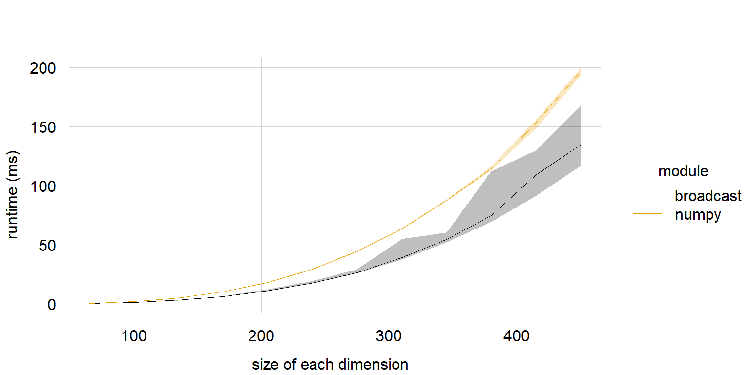
# 3d array #
print("3d")
gc.disable()
dimsizes = np.arange(65, 451, 35)
median_np = np.zeros(len(dimsizes))
q1_np = np.zeros(len(dimsizes))
q3_np = np.zeros(len(dimsizes))
durations = np.zeros(100)
for i in range(0, len(dimsizes)):
print(i)
n = dimsizes[i]
adims = (n, 1, n)
bdims = (1, n, 1)
x = np.random.random_sample(adims)
y = np.random.random_sample(bdims)
for j in range(0, len(durations)):
t1_start = perf_counter()
myfunc(x, y)
t1_stop = perf_counter()
durations[j] = (t1_stop-t1_start) * 1000
durations2 = durations[10:]
median_np[i] = np.median(durations2)
q1_np[i] = np.quantile(durations2, 0.25)
q3_np[i] = np.quantile(durations2, 0.75)
gc.collect()
np.savetxt("bm_py_3d_median.txt", median_np)
np.savetxt("bm_py_3d_q1.txt", q1_np)
np.savetxt("bm_py_3d_q3.txt", q3_np)
# end 3d array #
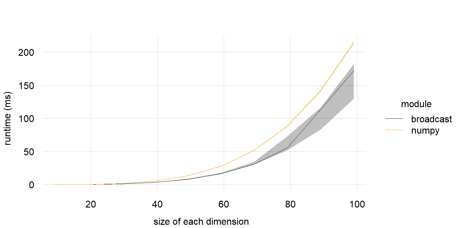
# 4d array #
print("4d")
gc.disable()
dimsizes = np.arange(9, 100, 10)
median_np = np.zeros(len(dimsizes))
q1_np = np.zeros(len(dimsizes))
q3_np = np.zeros(len(dimsizes))
durations = np.zeros(100)
for i in range(0, len(dimsizes)):
print(i)
n = dimsizes[i]
adims = (n, 1, n, 1)
bdims = (1, n, 1, n)
x = np.random.random_sample(adims)
y = np.random.random_sample(bdims)
for j in range(0, len(durations)):
t1_start = perf_counter()
myfunc(x, y)
t1_stop = perf_counter()
durations[j] = (t1_stop-t1_start) * 1000
durations2 = durations[10:]
median_np[i] = np.median(durations2)
q1_np[i] = np.quantile(durations2, 0.25)
q3_np[i] = np.quantile(durations2, 0.75)
gc.collect()
np.savetxt("bm_py_4d_median.txt", median_np)
np.savetxt("bm_py_4d_q1.txt", q1_np)
np.savetxt("bm_py_4d_q3.txt", q3_np)
# end 4d array #
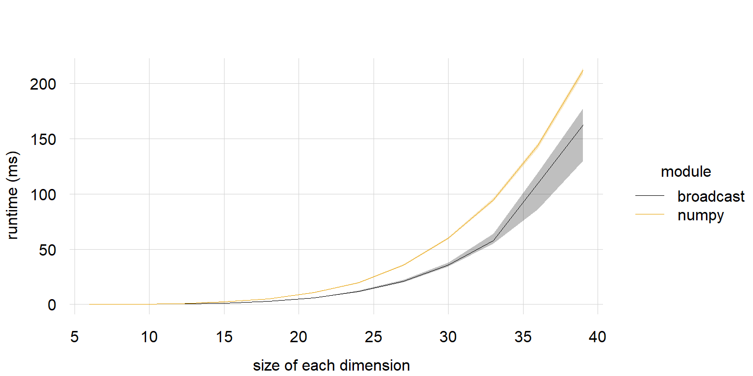
# 5d array #
print("5d")
gc.disable()
dimsizes = np.arange(6, 40, 3)
median_np = np.zeros(len(dimsizes))
q1_np = np.zeros(len(dimsizes))
q3_np = np.zeros(len(dimsizes))
durations = np.zeros(100)
for i in range(0, len(dimsizes)):
print(i)
n = dimsizes[i]
adims = (n, 1, n, 1, n)
bdims = (1, n, 1, n, 1)
x = np.random.random_sample(adims)
y = np.random.random_sample(bdims)
for j in range(0, len(durations)):
t1_start = perf_counter()
myfunc(x, y)
t1_stop = perf_counter()
durations[j] = (t1_stop-t1_start) * 1000
durations2 = durations[10:]
median_np[i] = np.median(durations2)
q1_np[i] = np.quantile(durations2, 0.25)
q3_np[i] = np.quantile(durations2, 0.75)
gc.collect()
np.savetxt("bm_py_5d_median.txt", median_np)
np.savetxt("bm_py_5d_q1.txt", q1_np)
np.savetxt("bm_py_5d_q3.txt", q3_np)
# end 5d array #
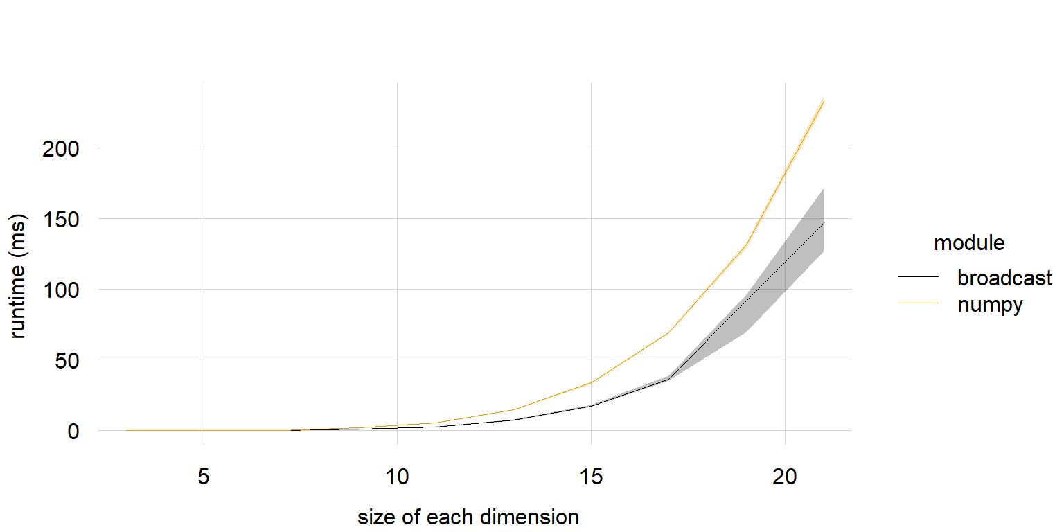
# 6d array #
print("6d")
gc.disable()
dimsizes = np.arange(3, 22, 2)
median_np = np.zeros(len(dimsizes))
q1_np = np.zeros(len(dimsizes))
q3_np = np.zeros(len(dimsizes))
durations = np.zeros(100)
for i in range(0, len(dimsizes)):
print(i)
n = dimsizes[i]
adims = (n, 1, n, 1, n, 1)
bdims = (1, n, 1, n, 1, n)
x = np.random.random_sample(adims)
y = np.random.random_sample(bdims)
for j in range(0, len(durations)):
t1_start = perf_counter()
myfunc(x, y)
t1_stop = perf_counter()
durations[j] = (t1_stop-t1_start) * 1000
durations2 = durations[10:]
median_np[i] = np.median(durations2)
q1_np[i] = np.quantile(durations2, 0.25)
q3_np[i] = np.quantile(durations2, 0.75)
gc.collect()
np.savetxt("bm_py_6d_median.txt", median_np)
np.savetxt("bm_py_6d_q1.txt", q1_np)
np.savetxt("bm_py_6d_q3.txt", q3_np)
# end 5d array #
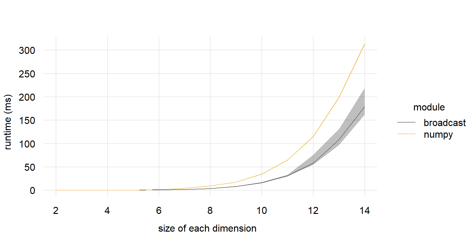
# 7d array #
print("7d")
gc.disable()
dimsizes = np.arange(2, 15, 1)
median_np = np.zeros(len(dimsizes))
q1_np = np.zeros(len(dimsizes))
q3_np = np.zeros(len(dimsizes))
durations = np.zeros(100)
for i in range(0, len(dimsizes)):
print(i)
n = dimsizes[i]
adims = (n, 1, n, 1, n, 1, n)
bdims = (1, n, 1, n, 1, n, 1)
x = np.random.random_sample(adims)
y = np.random.random_sample(bdims)
for j in range(0, len(durations)):
t1_start = perf_counter()
myfunc(x, y)
t1_stop = perf_counter()
durations[j] = (t1_stop-t1_start) * 1000
durations2 = durations[10:]
median_np[i] = np.median(durations2)
q1_np[i] = np.quantile(durations2, 0.25)
q3_np[i] = np.quantile(durations2, 0.75)
gc.collect()
np.savetxt("bm_py_7d_median.txt", median_np)
np.savetxt("bm_py_7d_q1.txt", q1_np)
np.savetxt("bm_py_7d_q3.txt", q3_np)
# end 7d array #