Standard Evaluated Versions of Some Common Expression-Evaluation Functions

The with_pro() and aes_pro() functions are standard-evaluated versions of the expression-evaluation functions with and ggplot2::aes, respectively.

These alternative functions are more programmatically friendly:
They use proper standard evaluation, through the usage of one-sided formulas, instead of non-standard evaluation, tidy evaluation, or similar programmatically unfriendly evaluations.

Usage

with_pro(data, form)

aes_pro(...)

Arguments

data: a list or data.frame.
form: a one-sided formula giving the expression to evaluate in with_pro.
If the formula has an environment, that environment is used to find any variables or objects not present in data.
...: arguments to be passed to ggplot2::aes, but given as one-sided formulas.

Value

For with_pro(): see with.
For aes_pro(): see ggplot2::aes.

Details

The aes_pro() function is the standard evaluated alternative to ggplot2::aes.
Due to the way aes_pro() is programmed, it should still work when tidy evaluation changes in 'ggplot2'.
To support functions in combinations with references of the variables, the input used here are formula inputs, rather than string inputs.
See the Examples section below.

Note

The with_pro() function, like the original with function, is made for primarily for convenience.
When using modelling or graphics functions with an explicit data argument (and typically using formulas), it is typically preferred to use the data argument of that function, rather than to use either
with(data, ...) or with_pro(data, ...).

Non-Standard Evaluation

Non-Standard Evaluation (sometimes abbreviated as "NSE"), is somewhat controversial.
Consider the following example:

aplot <- "ggplot2"
library(aplot)

What package will be attached? It will not be 'ggplot2', nor will an error occur. Instead, the package 'aplot' will be attached.
This is due to evaluating the expression 'aplot' as a quoted expression, instead of evaluating the contents (i.e. string or formula) of the variable. In other words: Non-Standard Evaluation.

Regular Standard Evaluation does not have the above problem.

Examples

requireNamespace("ggplot2")


d <- import_data("ggplot2", "mpg")

# mutate data:
myform <- ~ displ + cyl + cty + hwy
d$mysum <- with_pro(d, myform)
summary(d)
#>     manufacturer       model         displ            year           cyl       
#>  Length   :234   Length   :234   Min.   :1.600   Min.   :1999   Min.   :4.000  
#>  N.unique : 15   N.unique : 38   1st Qu.:2.400   1st Qu.:1999   1st Qu.:4.000  
#>  N.blank  :  0   N.blank  :  0   Median :3.300   Median :2004   Median :6.000  
#>  Min.nchar:  4   Min.nchar:  2   Mean   :3.472   Mean   :2004   Mean   :5.889  
#>  Max.nchar: 10   Max.nchar: 22   3rd Qu.:4.600   3rd Qu.:2008   3rd Qu.:8.000  
#>                                  Max.   :7.000   Max.   :2008   Max.   :8.000  
#>        trans            drv           cty             hwy       
#>  Length   :234   Length   :234   Min.   : 9.00   Min.   :12.00  
#>  N.unique : 10   N.unique :  3   1st Qu.:14.00   1st Qu.:18.00  
#>  N.blank  :  0   N.blank  :  0   Median :17.00   Median :24.00  
#>  Min.nchar:  8   Min.nchar:  1   Mean   :16.86   Mean   :23.44  
#>  Max.nchar: 10   Max.nchar:  1   3rd Qu.:19.00   3rd Qu.:27.00  
#>                                  Max.   :35.00   Max.   :44.00  
#>          fl            class         mysum      
#>  Length   :234   Length   :234   Min.   :33.70  
#>  N.unique :  5   N.unique :  7   1st Qu.:43.10  
#>  N.blank  :  0   N.blank  :  0   Median :50.15  
#>  Min.nchar:  1   Min.nchar:  3   Mean   :49.66  
#>  Max.nchar:  1   Max.nchar: 10   3rd Qu.:54.08  
#>                                  Max.   :84.90  

# plotting data:
x <- ~ cty
y <- ~ sqrt(hwy)
color <- ~ drv

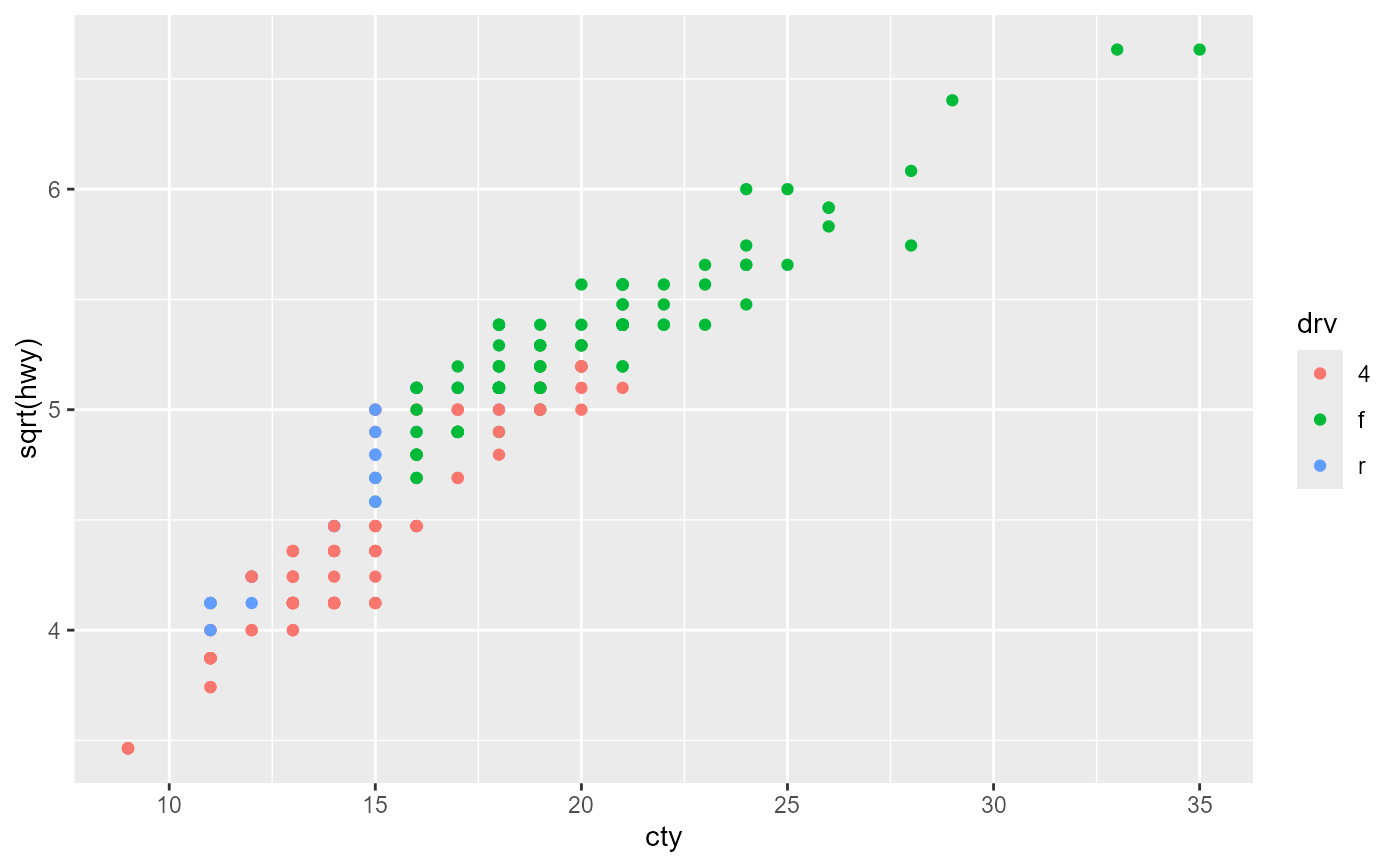
ggplot2::ggplot(d, aes_pro(x, y, color = color)) +
  ggplot2::geom_point()